
This page is the “theory” version of the topic; for applied RL framing, see the Hugging Face Deep RL notes. This revision adds Python, tables, images, and footnotes so you can see how math-heavy posts look when they’re not pretending to be short.1
Shannon entropy
Shannon’s central question (1948): how do you quantify information? His answer: information is the reduction of uncertainty. If I tell you something you already knew, I’ve given you zero information. If I tell you something surprising, I’ve given you a lot.
Formally, the entropy of a random variable \(X\) with possible outcomes \(x_1, \dots, x_n\):
\[H(X) = -\sum_{i} p(x_i) \log_2 p(x_i)\]
Entropy is maximized when all outcomes are equally likely (maximum uncertainty) and minimized (zero) when the outcome is deterministic. For a fair coin: \(H = -2 \times 0.5 \log_2(0.5) = 1\) bit. For a biased coin (99% heads): \(H \approx 0.08\) bits. The biased coin carries less information per flip because you already know what’s probably going to happen.
Quick reference — Bernoulli entropy
| \(P(X=1)\) | \(H(X)\) bits (base-2) | vibe |
|---|---|---|
| 0.5 | 1.000 | fair |
| 0.99 | ~0.081 | boring |
| 0.01 | ~0.081 | also boring (symmetry) |
| 0.0 or 1.0 | 0 | deterministic |
Takeaway: “surprise” and “information” are the same currency — measured in bits when you use \(\log_2\).2
Tiny Python sanity check
import math
from typing import Iterable

def entropy_bits(p: Iterable[float]) -> float:
    """Shannon entropy in bits for a discrete distribution."""
    return -sum(
        pi * math.log2(pi)
        for pi in p
        if pi > 0.0
    )

print(entropy_bits([0.5, 0.5]))          # 1.0
print(entropy_bits([0.99, 0.01]))        # ~0.0808
Cross-entropy
The cross-entropy between a true distribution \(p\) and a model distribution \(q\):
\[H(p, q) = -\sum_{i} p(x_i) \log q(x_i)\]
This is the loss function used in virtually all classification tasks in ML. When \(q = p\), cross-entropy equals entropy (the minimum). When \(q\) diverges from \(p\), cross-entropy increases. Training minimizes cross-entropy, which pushes the model’s predicted distribution toward the true distribution.
Numerical hygiene (footnote-sized lecture)
In code, you rarely compute log(0) directly — you clamp, or you use the built-in stabilized loss.3
import torch
import torch.nn.functional as F

# logits: raw scores from the last linear layer; target: class indices
def ce_loss(logits: torch.Tensor, target: torch.Tensor) -> torch.Tensor:
    return F.cross_entropy(logits, target)  # log-softmax + NLL, stabilized internally
KL divergence
The Kullback-Leibler divergence measures how different \(q\) is from \(p\):
\[D_{KL}(p \| q) = \sum_{i} p(x_i) \log \frac{p(x_i)}{q(x_i)} = H(p, q) - H(p)\]
Since \(H(p)\) is constant with respect to \(q\), minimizing cross-entropy is equivalent to minimizing KL divergence. This is why cross-entropy is used as a loss: it’s a proxy for “how wrong is the model.”
Important: KL divergence is NOT symmetric. \(D_{KL}(p \| q) \neq D_{KL}(q \| p)\). This asymmetry has practical consequences:
- Mode-covering (\(D_{KL}(p \| q)\)): the model tries to cover all modes of \(p\), even at the cost of spreading probability mass to unlikely regions. This is what variational inference typically minimizes.
- Mode-seeking (\(D_{KL}(q \| p)\)): the model collapses to a single mode of \(p\), ignoring others. This is what GANs tend to do.
Nested blockquote, because this point confuses everyone at least once:
Remember: KL is an expectation under \(p\) of log-ratios.
If you swap which distribution sits “under the expectation,” you get a different objective — not “the same thing but tweaked.”
Mutual information
The mutual information between two variables \(X\) and \(Y\):
\[I(X; Y) = H(X) - H(X|Y) = H(Y) - H(Y|X)\]
It measures how much knowing one variable reduces uncertainty about the other. If \(X\) and \(Y\) are independent, \(I(X;Y) = 0\). If knowing \(X\) completely determines \(Y\), then \(I(X;Y) = H(Y)\).
This shows up in feature selection (which features carry the most information about the target), representation learning (InfoNCE loss), and decision trees (information gain is mutual information between a feature and the class label).
Figure: classic RL diagram (caption pattern)
Cross-linking visuals helps when you’re bouncing between “information theory” and “agents in environments”:
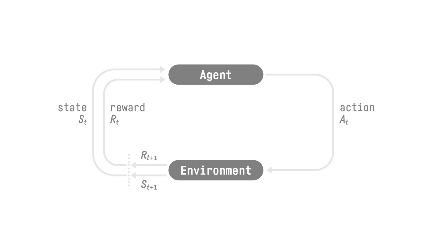 The RL loop — states, actions, rewards — same picture as in the HF RL notes, different surrounding prose.
 Legacy screenshot kept around to test PNG + caption styling on long pages.
Why this matters
Shannon’s framework provides a rigorous language for talking about learning. Training a model is reducing entropy. Overfitting is memorizing noise instead of structure. Compression and prediction are the same problem viewed from different angles (a good predictor is a good compressor, and vice versa). Information theory doesn’t tell you how to learn, but it tells you what learning means.
Checklist: translating theory to debugging questions
- Calibration: Are my predicted probabilities meaningful — or just ranking scores?4
- Bottlenecks: Is mutual information between representation and label actually non-trivial?
- Regularization: Am I penalizing capacity or penalizing noise fitting — different fixes.
# Not information theory — just the vibe of "measure everything"
python - <<'PY'
import math
for p in [0.5, 0.9, 0.99]:
    print(p, -p*math.log2(p) - (1-p)*math.log2(1-p))
PY
Table stress (entropy, code, dollars)
| Object | Definition | One-liner |
|---|---|---|
| Entropy | \(H(X) = -\sum_x p(x)\log p(x)\) | -(p * p.log()).sum() in PyTorch |
| Cross-entropy | \(H(p,q) = -\sum_x p(x)\log q(x)\) | F.cross_entropy(logits, y) |
| KL | \(D_{\mathrm{KL}}(p\|q) = H(p,q) - H(p)\) | often implicit in training |
Footer: all three columns mix TeX and backticks.
| Paper / book | Price (fake) | Why it’s in the pile |
|---|---|---|
| Cover & Thomas | $45 used | Chapters 2–8 — treat as reference, not a novel |
| MacKay (free PDF) | $0 | Download, grep, love |
| This note | $0 + your time | Long cell: information theory is the language for “how surprised should I be” and “how wrong is my model,” and tables are where you compare definitions side-by-side without scrolling three screens of prose. |
Footer: literal \$ for fake prices + long third column.
| \(p\) | \(H_2(p)\) bits | python |
|---|---|---|
| 0.5 | 1.0 | -sum(p*log2(p) for p in [0.5,0.5]) |
| 0.9 | \(\approx 0.469\) | entropy_bits([0.9, 0.1]) from earlier |
Counted tables: expect “Table 1 —”.
| Symbol | Meaning |
|---|---|
| \(\log\) | default base in ML is often natural log (nats); bits need \(\log_2\) |
| \(\mathbb{1}{\cdot}\) | indicator — 1 if true, else 0 |
Second caption in block — “Table 2 —”.
Further reading (external): MacKay’s Information Theory, Inference, and Learning Algorithms (free PDF) — famously readable. For ML-heavy treatment: Bishop’s Pattern Recognition and ML (chapters on entropy/KL in discrete settings).
Scope: intuition + definitions + a few lines of code — not a full course. For depth: Cover & Thomas, Elements of Information Theory. ↩
You can use nats (\(\ln\)) instead; ML papers often implicitly use nats when they write
logwithout specifying a base. ↩See log-sum-exp trick — related to how softmax + cross-entropy are implemented safely in frameworks. ↩
Calibration is not the same as accuracy — see calibration (statistics). ↩